论文链接:High-Resolution Image Synthesis
with Latent Diffusion Models
官方实现:CompVis/latent-diffusion CompVis/stable-diffusion
这一篇文章的内容是 Latent Diffusion Models(LDM),也就是大名鼎鼎的
Stable
Diffusion。先前的扩散模型一直面临的比较大的问题是采样空间太大,学习的噪声维度和图像的维度是相同的。当进行高分辨率图像生成时,需要的计算资源会急剧增加,虽然
DDIM 等工作已经对此有所改善,但效果依然有限。Stable Diffusion
的方法非常巧妙,其把扩散过程转换到了低维度的隐空间中,解决了这个问题。
方法介绍
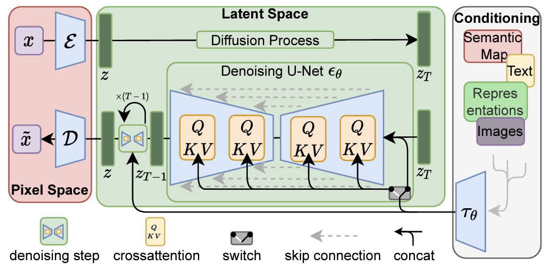
本方法的整体结构如下图所示,主要分为三部分:最左侧的红框对应于感知图像压缩,中间的绿框对应
Latent Diffusion
Models,右侧的白框表示生成条件,下面将分别介绍这三个部分。
感知图像压缩
LDM
把图像生成过程从原始的图像像素空间转换到了一个隐空间,具体来说,对于一个维度为
\(\mathbf{x}\in\mathbb{R}^{H\times W\times
3}\) 的 RGB 图像,可以使用一个 encoder \(\mathcal{E}\) 将其转换为隐变量 \(\mathbf{z}=\mathcal{E}(\mathbf{x})\) ,也可以用一个
decoder \(\mathcal{D}\)
将其从隐变量转换回像素空间 \(\tilde{\mathbf{x}}=\mathcal{D}(\mathcal{E}(\mathbf{x}))\) 。在转换时会将图像下采样,作者测试了一系列下采样倍数
\(f\in\{1, 2, 4, 8, 16,
32\}\) ,发现下采样 4-16 倍的时候可以比较好地权衡效率和质量。
在进行图像压缩时,为了防止压缩后的空间是某个高方差的空间,需要进行正则化。作者使用了两种正则化,第一种是
KL-正则化,也就是将隐变量和标准高斯分布使用一个 KL
惩罚项进行正则化;第二种是 VQ-正则化,也就是使用一个 vector quantization
层进行正则化。
Latent Diffusion Models
实际上 latent diffusion models
和普通的扩散模型没有太大区别,只是因为从像素空间变到了隐空间,所以维度降低了。训练的优化目标也没有太大变化,普通的扩散模型优化目标为:
\[
L_\textrm{DM}=\mathbb{E}_{\mathbf{x},\epsilon\sim\mathcal{N}(0,1),t}\left[||\epsilon-\epsilon_\theta(\mathbf{x}_t,t)||_2^2\right]
\] 而 Latent Diffusion Models 的优化目标只是套了一层
autoencoder: \[
L_\textrm{LDM}=\mathbb{E}_{\textcolor{red}{\mathcal{E}(\mathbf{x})},\epsilon\sim\mathcal{N}(0,1),t}\left[||\epsilon-\epsilon_\theta(\mathbf{x}_t,t)||_2^2\right]
\] 在采样时,首先从隐空间随机采样噪声,在去噪后再用 decoder
转换到像素空间即可。
条件生成
为了进行条件生成,需要学习 \(\epsilon_\theta(\mathbf{x}_t,t,y)\) ,这里使用的方法是在去噪网络中加入
cross attention 层,条件通过交叉注意力注入。在计算注意力时,\(\mathbf{z}\) 为 Query、\(y\) 为 Key 和 Value,具体的内容已经在 Classifier-Free
Guidance 的文章中 介绍过了,对具体细节感兴趣的读者可以去看一下。
代码解读
Stable Diffusion 有两套主流的代码实现,第一种是 CompVis
的官方实现,第二种是 huggingface
的实现。这里的代码解读都以文生图任务为例。
CompVis 的实现
这个实现的代码比较分散,层次结构不太好梳理,不过可以照着配置文件看各部分都在哪里。这个配置文件有点类似
openmmlab 的那套框架的写法,例如文生图的配置文件
models/ldm/text2img256/config.yaml:
1
2
3
4
5
6
7
8
9
model: target: ldm.models.diffusion.ddpm.LatentDiffusion params: unet_config: target: ldm.modules.diffusionmodules.openaimodel.UNetModel first_stage_config: target: ldm.models.autoencoder.VQModelInterface cond_stage_config: target: ldm.modules.encoders.modules.BERTEmbedder
无关的内容都略去,可以看到顶层的模块是
LatentDiffusion,去噪网络是 UNetModel、encoder
是 VQModelInterface、文本编码器是
BERTEmbedder。
这里主要还是关注 LatentDiffusion
的采样过程。具体的采样代码位于 LatentDiffusion.sample:
1
2
3
4
5
6
7
8
9
10
11
12
13
14
15
16
17
18
19
@torch.no_grad() def sample (self, cond, batch_size=16 , return_intermediates=False , x_T=None , verbose=True , timesteps=None , quantize_denoised=False , mask=None , x0=None , shape=None , **kwargs ): if shape is None : shape = (batch_size, self.channels, self.image_size, self.image_size) if cond is not None : if isinstance (cond, dict ): cond = {key: cond[key][:batch_size] if not isinstance (cond[key], list ) else list (map (lambda x: x[:batch_size], cond[key])) for key in cond} else : cond = [c[:batch_size] for c in cond] if isinstance (cond, list ) else cond[:batch_size] return self.p_sample_loop(cond, shape, return_intermediates=return_intermediates, x_T=x_T, verbose=verbose, timesteps=timesteps, quantize_denoised=quantize_denoised, mask=mask, x0=x0)
可以看到实际的采样过程并不是在这一层进行,这一层只进行了一些封装,例如采样的大小以及条件的数据格式等等,具体的采样则是在
p_sample_loop 中进行的:
1
2
3
4
5
6
7
8
9
@torch.no_grad() def p_sample_loop (self, cond, shape, timesteps=None ): iterator = tqdm(reversed (range (0 , timesteps)), desc='Sampling t' , total=timesteps) if verbose else reversed (range (0 , timesteps)) for i in iterator: ts = torch.full((b,), i, device=device, dtype=torch.long) img = self.p_sample(img, cond, ts, clip_denoised=self.clip_denoised, quantize_denoised=quantize_denoised) return img
去掉一堆杂七杂八的代码之后可以发现在 p_sample_loop
中是一个循环,也就对应于一步步进行降噪的过程,具体的降噪在
p_sample 中实现:
1
2
3
4
5
6
7
8
9
10
11
12
13
14
15
16
17
18
@torch.no_grad() def p_sample (self, x, c, t, clip_denoised=False , repeat_noise=False , return_codebook_ids=False , quantize_denoised=False , return_x0=False , temperature=1. , noise_dropout=0. , score_corrector=None , corrector_kwargs=None ): b, *_, device = *x.shape, x.device outputs = self.p_mean_variance(x=x, c=c, t=t, clip_denoised=clip_denoised, return_codebook_ids=return_codebook_ids, quantize_denoised=quantize_denoised, return_x0=return_x0, score_corrector=score_corrector, corrector_kwargs=corrector_kwargs) model_mean, _, model_log_variance = outputs noise = noise_like(x.shape, device, repeat_noise) * temperature if noise_dropout > 0. : noise = torch.nn.functional.dropout(noise, p=noise_dropout) nonzero_mask = (1 - (t == 0 ).float ()).reshape(b, *((1 ,) * (len (x.shape) - 1 ))) return model_mean + nonzero_mask * (0.5 * model_log_variance).exp() * noise
在 p_sample 中,首先用模型预测出了均值和方差(也就是
p_mean_variance,这里就不展开讲了),然后进行了去噪。
综合上述分析来看,如果看原始代码,可能会觉得非常混乱,但是其实去掉不重要的内容之后,核心的代码并不算非常多。这里没有展开具体的
p_mean_variance 内部的内容,在 CompVis 的框架中,定义了很多
diffusion 中常用的常量(例如
alphas_cumprod、sqrt_recipm1_alphas_cumprod
等)和方法(例如
q_mean_variance、p_mean_variance
等),后续我应该还会写一篇文章专门介绍这些内容,这里暂时略过,只需要知道最顶层的
p_mean_variance 是预测了均值和方差即可。
huggingface 的实现
相比于 CompVis 的实现,huggingface 的实现更加工程化一点,相关的在
diffusers
库中。这个库主要包括三大类元素:models(各种神经网络的实现,unet、vae
等)、schedulers(diffusion 相关的操作,加噪去噪等)、pipelines(high
level 封装,相当于 models+schedulers,这个应该是方便用户直接用的)。
这里直接看
diffusers/pipelines/stable_diffusion/pipeline_stable_diffusion.py
的采样过程,定义在 __call__ 函数中:
1
2
3
4
5
6
7
8
9
10
11
12
13
14
15
16
17
18
19
20
21
22
23
24
25
26
27
28
29
30
31
@torch.no_grad() @replace_example_docstring(EXAMPLE_DOC_STRING ) def __call__ ( self, prompt: Union [str , List [str ]] = None , height: Optional [int ] = None , width: Optional [int ] = None , num_inference_steps: int = 50 , timesteps: List [int ] = None , sigmas: List [float ] = None , guidance_scale: float = 7.5 , negative_prompt: Optional [Union [str , List [str ]]] = None , num_images_per_prompt: Optional [int ] = 1 , eta: float = 0.0 , generator: Optional [Union [torch.Generator, List [torch.Generator]]] = None , latents: Optional [torch.Tensor] = None , prompt_embeds: Optional [torch.Tensor] = None , negative_prompt_embeds: Optional [torch.Tensor] = None , ip_adapter_image: Optional [PipelineImageInput] = None , ip_adapter_image_embeds: Optional [List [torch.Tensor]] = None , output_type: Optional [str ] = "pil" , return_dict: bool = True , cross_attention_kwargs: Optional [Dict [str , Any ]] = None , guidance_rescale: float = 0.0 , clip_skip: Optional [int ] = None , callback_on_step_end: Optional [ Union [Callable [[int , int , Dict ], None ], PipelineCallback, MultiPipelineCallbacks] ] = None , callback_on_step_end_tensor_inputs: List [str ] = ["latents" ], **kwargs,
可以看到参数实在是非常的多,我们在这里不关注工程的部分,只关注核心的逻辑。这里的第一个需要关注的点是对生成条件进行编码:
1
2
3
4
5
6
7
8
9
10
11
12
13
14
15
16
prompt_embeds, negative_prompt_embeds = self.encode_prompt( prompt, device, num_images_per_prompt, self.do_classifier_free_guidance, negative_prompt, prompt_embeds=prompt_embeds, negative_prompt_embeds=negative_prompt_embeds, lora_scale=lora_scale, clip_skip=self.clip_skip, ) if self.do_classifier_free_guidance: prompt_embeds = torch.cat([negative_prompt_embeds, prompt_embeds])
这里实际上还有 LoRA 和 IP-Adaptor
相关的处理,暂时省略。可以看到这里对生成的 prompt
进行了编码,并且不仅有正常的 prompt,还有 negative 的 prompt,这是为了做
classifier-free guidance。并且由于两个 prompt 需要分别推理,这里还将其在
batch 维度拼接,来进行并行化。随后获取 timesteps:
1
2
3
timesteps, num_inference_steps = retrieve_timesteps( self.scheduler, num_inference_steps, device, timesteps, sigmas )
然后初始化噪声,这个就相当于 \(\mathbf{x}_T\) :
1
2
3
4
5
6
7
8
9
10
11
num_channels_latents = self.unet.config.in_channels latents = self.prepare_latents( batch_size * num_images_per_prompt, num_channels_latents, height, width, prompt_embeds.dtype, device, generator, latents, )
上边准备了 \(\mathbf{x}\) 、timestep
以及 condition,现在就可以正式进行生成了:
1
2
3
4
5
6
7
8
9
10
11
12
13
14
15
16
17
18
19
20
21
22
23
24
25
26
num_warmup_steps = len (timesteps) - num_inference_steps * self.scheduler.order self._num_timesteps = len (timesteps) with self.progress_bar(total=num_inference_steps) as progress_bar: for i, t in enumerate (timesteps): latent_model_input = torch.cat([latents] * 2 ) if self.do_classifier_free_guidance else latents latent_model_input = self.scheduler.scale_model_input(latent_model_input, t) noise_pred = self.unet( latent_model_input, t, encoder_hidden_states=prompt_embeds, timestep_cond=timestep_cond, cross_attention_kwargs=self.cross_attention_kwargs, added_cond_kwargs=added_cond_kwargs, return_dict=False , )[0 ] if self.do_classifier_free_guidance: noise_pred_uncond, noise_pred_text = noise_pred.chunk(2 ) noise_pred = noise_pred_uncond + self.guidance_scale * (noise_pred_text - noise_pred_uncond) if self.do_classifier_free_guidance and self.guidance_rescale > 0.0 : noise_pred = rescale_noise_cfg(noise_pred, noise_pred_text, guidance_rescale=self.guidance_rescale) latents = self.scheduler.step(noise_pred, t, latents, **extra_step_kwargs, return_dict=False )[0 ]
可以看到有一些为了 classifier-free guidance
进行的处理,其他的都是正常 diffusion
的操作。最后将隐变量解码回像素空间得到生成结果:
1 image = self.vae.decode(latents / self.vae.config.scaling_factor, return_dict=False , generator=generator)[0 ]
总结
最近看了这么多文章,感觉比较成功的 researcher
的工作都是连贯的。就像宋飏研究 sliced score matching,然后紧随其后做出了
score-based generative model;又如 OpenAI 训出 CLIP 然后基于 CLIP
做了一系列文生图的工作。今天这篇文章看起来也是 CompVis 把 VQGAN 迁移到
diffusion models
上的成果,感觉对平时做研究的启发还是很大的,我个人一直以来研究方向都比较摇摆不定,也应该反思学习一下。
参考资料:
diffusion
model(五):LDM: 在隐空间用diffusion model合成高质量图片 扩散模型(六)|
Stable Diffusion