论文链接:Improved
Denoising Diffusion Probabilistic Models
在前边两篇文章中我们学习了 DDPM 和 DDIM,这篇文章介绍的是 Improved
DDPM,是一个针对 DDPM 生成效果进行改进的工作。
虽然 DDPM 在生成任务上取得了不错的效果,但如果使用一些 metric 对 DDPM
进行评价,就会发现其虽然能在 FID 和 Inception Score
上获得不错的效果,但在负对数似然(Negative
Log-likelihood,NLL)这个指标上表现不够好。根据 VQ-VAE2 文章中的观点,NLL
上的表现体现的是模型捕捉数据整体分布的能力。而且有工作表明即使在 NLL
指标上仅有微小的提升,就会在生成效果和特征表征能力上有很大的提升。
Improved DDPM 主要是针对 DDPM
的训练过程进行改进,主要从两个方面进行改进:
不使用 DDPM 原有的固定方差,而是使用可学习的方差;
改进了加噪过程,使用余弦形式的 Scheduler,而不是线性
Scheduler。
可学习的方差
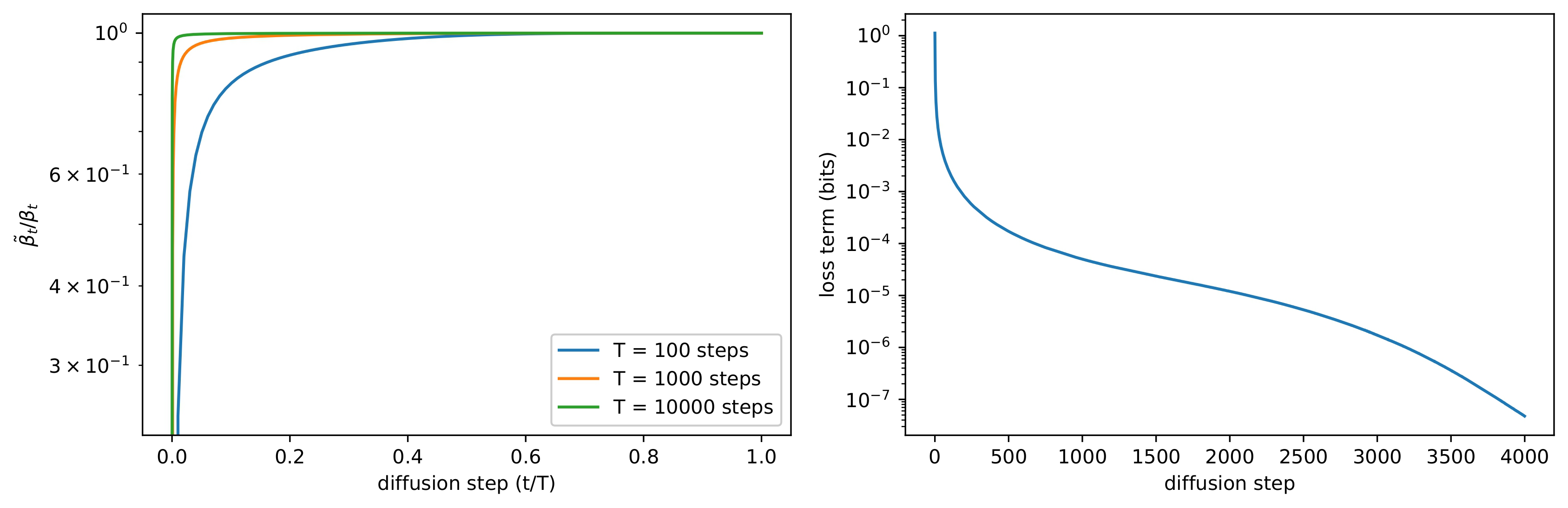
我们知道 DDPM 规定了一系列固定的 \(\beta_t\) 作为方差,并且将 \(\sigma^2_t\) 分别取为 \(\sigma_t^2=\beta_t\) 和 \(\sigma_t^2=\tilde{\beta}_t\)
得到的结果差别并不大。之所以会出现这种情况,可以从下面的左图中看出大致的原因,只有在扩散过程最开始的时候
\(\tilde{\beta}_t\) 才和 \(\beta_t\)
有比较大的差距,而当扩散步骤增大时,这两者基本上没有区别。这说明当扩散步骤足够大的时候,\(\sigma_t\)
的选取对采样的质量影响不大,也就是说这种情况下,模型的平均值 \(\mu_\theta(\mathbf{x}_t,t)\) 比方差 \(\Sigma_\theta(\mathbf{x}_t,t)\)
更能决定生成的分布。
虽然上边这个发现从一定程度上可以说明方差的选取并不重要。但再来看一下下面的右图,可以发现在扩散的过程中,最初的几步扩散对
VLB 的影响是最大的,在这几个步骤里 \(\sigma_t\)
依然是有一定的作用的,因此作者认为可以通过选取比较好的方差来获得更好的
log-likelihood。从这个角度出发,作者引入了一个可学习的方差。
既然要选择一个可学习的方差,那么现在的问题就变成了应该如何选取一个合适的方差。这个工作的作者认为因为方差的变化范围比较小,不太容易用神经网络进行学习,所以实际上使用的方差是对
\(\beta_t\) 和 \(\tilde{\beta}_t\) 进行插值的结果: \[
\Sigma_\theta(\mathbf{x}_t,t)=\exp(v\log\beta_t+(1-v)\log\tilde\beta_t)
\] 在实际训练的时候并没有对 \(v\)
进行约束,所以理论上来说最后的方差不一定在这两者之间,不过经过实验发现没有出现这个情况。
Cosine Noise Schedule
本文的作者发现线性的 \(\beta_t\)
对于高分辨率图像效果不错,但对于低分辨率的图像表现不佳。在之前的文章中我们提到过,在
DDPM 加噪的时候 \(\beta_t\)
是从一个比较小的数值逐渐增加到比较大的数值的,因为如果最开始的时候加入很大的噪声,会严重破坏图像信息,不利于图像的学习。在这里应该也是相同的道理,因为低分辨率图像包含的信息本身就不多,虽然一开始使用了比较小的
\(\beta_t\) ,但线性的 schedule
对于这些低分辨率图像来说还是加噪比较快。
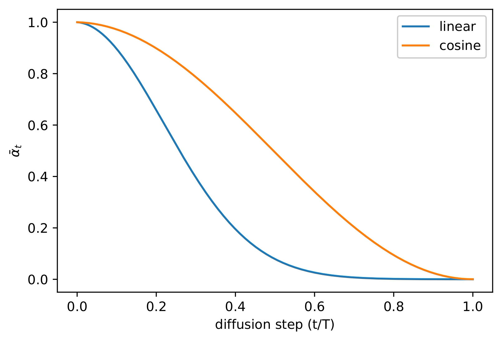
作者把方差用一种 cosine 的形式定义,不过并不是直接定义 \(\beta_t\) ,而是定义 \(\bar{\alpha}_t\) : \[
\bar{\alpha}_t=\frac{f(t)}{f(0)},\quad
f(t)=\cos\left(\frac{t/T+s}{1+s}\cdot\frac{\pi}{2}\right)^2
\] 这个 schedule 和线性 schedule 的比较如下图所示:
这个 schedule 在 \(t=0\) 和 \(t=T\)
附近都变化比较小,而在中间有一个接近于线性的下降过程,同时可以发现
cosine schedule 比 linear schedule
对信息的破坏更慢。这也印证了我们在前边提到的理论:在扩散开始的时候更加缓慢地加噪,可以得到更好的训练效果。除此之外设计这个
schedule 的时候作者也有一些比较细节的考虑,比如选取一个比较小的偏移量
\(s=8\times10^{-3}\) ,防止 \(\beta_t\) 在 \(t=0\) 附近过小,并且将 \(\beta_t\) 裁剪到 \(0.999\) 来防止 \(t=T\) 附近出现奇异点。
训练过程
最终训练使用的损失是两项损失的加权: \[
L_\mathrm{hybrid}=L_\mathrm{simple}+\lambda L_\mathrm{vlb}
\] 在这里,\(L_\mathrm{simple}\)
就是 DDPM 使用的 L2 损失:\(L_\mathrm{simple}=E_{t,\mathbf{x}_0,\epsilon}[||\epsilon-\epsilon_\theta(\mathbf{x}_t,t)||^2]\) ,而
\(L_\mathrm{vlb}\) 是用 VAE
的形式写出的损失函数: \[
\begin{aligned}
L_\mathrm{vlb}&=L_0+L_1+\cdots+L_{T-1}+L_T\\
L_0&=-\log p_\theta(\mathbf{x}_0|\mathbf{x}_1)\\
L_{t-1}&=D_{KL}(q(\mathbf{x}_{t-1}|\mathbf{x}_t,\mathbf{x}_0)||p_\theta(\mathbf{x}_{t-1}|\mathbf{x}_t))\\
L_T&=D_{KL}(q(\mathbf{x}_T|\mathbf{x}_0)||p(\mathbf{x}_T))
\end{aligned}
\] 为了防止 \(L_\mathrm{vlb}\)
影响 \(L_\mathrm{simple}\) ,这里使用了一个比较小的权重
\(\lambda=1\times10^{-3}\) ,并且对 VLB
损失中的均值项 \(\mu_\theta(\mathbf{x}_t,t)\) 进行了
stop-gradient,从而让 \(L_\mathrm{simple}\)
依然是均值的主要决定因素。
作者也表示最开始本来想直接优化 \(L_\mathrm{vlb}\) ,但是后来发现 \(L_\mathrm{vlb}\) 很难优化。作者分析认为
\(L_\mathrm{vlb}\) 的梯度比 \(L_\mathrm{hybrid}\) 更加
noisy,这是因为不同时间步的 VLB
损失大小不一(也就是上边那个损失曲线),均匀采样时间步 \(t\)
会引入比较多的噪音。为了解决这个问题,作者引入了一个重要性采样: \[
L_\mathrm{vlb}=E_{t\sim
p_t}\left[\frac{L_t}{p_t}\right],\quad\text{where}~p\propto\sqrt{E[L_t^2]}~\text{and}~\sum
p_t=1
\] 由于 \(E[L_t^2]\)
不能预先得知,并且在训练过程中会变化,实际上训练的时候会保存 10
项历史的损失,并且对此进行动态更新。这部分光看公式可能不太容易理解,可以参照下面代码实现部分的
ImportanceSampler
来看:具体的做法就是给每个时间步都保存了最近的 10
个历史损失,然后在采样时间步的时候,用所有保存的损失生成时间步的重要性分布,从分布里采样。除此之外这些损失还能用来计算出每个时间步的权重,在计算最终的损失的时候每个时间步的损失先乘以对应的权重,然后再进行加和得到整体的损失。
Improved DDPM 的代码实现
为了方便和 DDPM 的效果进行比较,我们依然继承在实现 DDPM
时所写代码的主要部分,仅改变其中部分处理。对于这里没有完全介绍的部分(比如训练参数、数据集等)可以移步这篇文章 查看,在文章的最后也给出了完整代码,被省略的部分也可以去看完整代码。
Cosine Noise Schedule
我们先从比较简单的部分开始实现,因为前文已经给出了 cosine noise
schedule 的公式,我们直接对着公式写出代码就可以了: \[
\begin{aligned}
\bar{\alpha}_t&=\frac{f(t)}{f(0)},\quad
f(t)=\cos\left(\frac{t/T+s}{1+s}\cdot\frac{\pi}{2}\right)^2\\
\beta_t&=1-\frac{\bar{\alpha}_t}{\bar{\alpha}_{t-1}}
\end{aligned}
\]
1
2
3
4
5
6
7
8
9
10
11
12
13
14
15
16
17
18
19
20
21
22
23
24
25
26
27
28
29
30
31
32
import mathimport torchfrom tqdm import tqdmfrom functools import partialdef make_betas_cosine_schedule ( num_diffusion_timesteps: int = 1000 , beta_max: float = 0.999 , s: float = 8e-3 , fn = lambda t: math.cos((t + s) / (1 + s) * math.pi / 2 ) ** 2 betas = [] for i in range (num_diffusion_timesteps): t1 = i / num_diffusion_timesteps t2 = (i + 1 ) / num_diffusion_timesteps betas.append(1.0 - fn(t2) / fn(t1)) return torch.tensor(betas, dtype=torch.float32).clamp_max(beta_max) class IDDPM : def __init__ ( self, num_diffusion_timesteps: int = 1000 , beta_max: float = 0.999 , ): self.num_diffusion_timesteps = num_diffusion_timesteps self.betas = make_betas_cosine_schedule(num_diffusion_timesteps, beta_max) self.alphas = 1.0 - self.betas self.alphas_cumprod = torch.cumprod(self.alphas, dim=0 ) self.alphas_cumprod_prev = torch.concat((torch.ones(1 ).to(self.alphas_cumprod), self.alphas_cumprod[:-1 ])) self.alphas_cumprod_next = torch.concat((self.alphas_cumprod[1 :], torch.zeros(1 ).to(self.alphas_cumprod))) self.timesteps = torch.arange(num_diffusion_timesteps - 1 , -1 , -1 )
可学习的方差
实现可学习方差非常简单,只需要把原来的 3 通道输出直接改成 6
通道就可以了,前三个通道表示学习的均值,后三个通道表示学习的方差:
1
2
3
4
5
6
7
8
9
10
11
12
13
14
15
16
17
18
19
20
21
22
23
24
25
from diffusers import UNet2DModelmodel = UNet2DModel( sample_size=config.image_size, in_channels=3 , out_channels=6 , layers_per_block=2 , block_out_channels=(128 , 128 , 256 , 256 , 512 , 512 ), down_block_types=( "DownBlock2D" , "DownBlock2D" , "DownBlock2D" , "DownBlock2D" , "AttnDownBlock2D" , "DownBlock2D" , ), up_block_types=( "UpBlock2D" , "AttnUpBlock2D" , "UpBlock2D" , "UpBlock2D" , "UpBlock2D" , "UpBlock2D" , ), )
采样过程
Improved DDPM 的加噪过程和 DDPM
是完全一样的,在这里就不赘述了,主要不同的是采样的过程。在采样过程中,均值的计算与
DDPM 也是完全一样,直接把之前写的 DDPM 均值计算 copy
过来就可以了。主要需要改动的是方差的计算部分,其实也比较简单直接,就是
DDPM 的方差直接和 \(\log\beta_t\) 和
\(\log\tilde{\beta}_t\)
直接加权。因为广播需要维度数量对齐,所以这里专门定义了一个对齐维度的函数。这里也贴一下公式方便参考:
\[
\begin{aligned}
\tilde{\beta}_t&=\frac{1-\bar{\alpha}_{t-1}}{1-\bar{\alpha}_t}\beta_t\\
\Sigma_\theta(\mathbf{x}_t,t)&=\exp(v\log\beta_t+(1-v)\log\tilde\beta_t)
\end{aligned}
\]
1
2
3
4
5
6
7
8
9
10
11
12
13
14
15
16
17
18
19
20
21
22
23
24
25
26
27
28
29
30
31
32
33
34
35
36
37
38
39
40
41
42
43
44
45
46
47
48
49
50
51
52
53
54
55
56
def extract (arr: torch.Tensor, timesteps: torch.Tensor, broadcast_shape: torch.Size ): arr = arr[timesteps] while len (arr.shape) < len (broadcast_shape): arr = arr.unsqueeze(-1 ) return arr.expand(broadcast_shape) class IDDPM : ... @torch.no_grad() def sample ( self, unet: UNet2DModel, batch_size: int , in_channels: int , sample_size: int , ): images = torch.randn((batch_size, in_channels, sample_size, sample_size), device=unet.device) betas = self.betas.to(unet.device) alphas = self.alphas.to(unet.device) alphas_cumprod = self.alphas_cumprod.to(unet.device) alphas_cumprod_prev = self.alphas_cumprod_prev.to(unet.device) timesteps = self.timesteps.to(unet.device) sqrt_recip_alphas_cumprod = (1.0 / alphas_cumprod) ** 0.5 sqrt_recipm1_alphas_cumprod = (1.0 / alphas_cumprod - 1.0 ) ** 0.5 posterior_variance = betas * (1.0 - alphas_cumprod_prev) / (1.0 - alphas_cumprod) posterior_log_variance_clipped = torch.log(torch.concat((posterior_variance[1 :2 ], posterior_variance[1 :]))) posterior_mean_coef1 = betas * alphas_cumprod_prev ** 0.5 / (1.0 - alphas_cumprod) posterior_mean_coef2 = (1.0 - alphas_cumprod_prev) * alphas ** 0.5 / (1.0 - alphas_cumprod) for timestep in tqdm(timesteps, desc='Sampling' ): _extract = partial(extract, timesteps=timestep, broadcast_shape=images.shape) preds: torch.Tensor = unet(images, timestep).sample pred_noises, pred_vars = torch.split(preds, in_channels, dim=1 ) x_0 = _extract(sqrt_recip_alphas_cumprod) * images - _extract(sqrt_recipm1_alphas_cumprod) * pred_noises mean = _extract(posterior_mean_coef1) * x_0.clamp(-1 , 1 ) + _extract(posterior_mean_coef2) * images if timestep > 0 : min_log = _extract(posterior_log_variance_clipped) max_log = _extract(torch.log(betas)) frac = (pred_vars + 1.0 ) / 2.0 log_variance = frac * max_log + (1.0 - frac) * min_log stddev = torch.exp(0.5 * log_variance) else : stddev = torch.zeros_like(timestep) epsilon = torch.randn_like(images) images = mean + stddev * epsilon images = (images / 2.0 + 0.5 ).clamp(0 , 1 ).cpu().permute(0 , 2 , 3 , 1 ).numpy() return images
模型训练
损失函数
训练的大部分代码都和 DDPM
一样,不一样的只有损失函数以及重要性采样。这里定义一个专门用来计算 IDDPM
的损失函数。损失函数共由两项组成,也就是 \(L_\mathrm{simple}\) 和 \(L_\mathrm{vlb}\) :
1
2
3
4
5
6
7
8
9
10
11
12
13
14
15
16
17
18
def training_losses ( iddpm: IDDPM, model: UNet2DModel, clean_images: torch.Tensor, noise: torch.Tensor, noisy_images: torch.Tensor, timesteps: torch.Tensor, vlb_weight: float = 1e-3 , _, channels, _, _ = noisy_images.shape pred: torch.Tensor = model(noisy_images, timesteps, return_dict=False )[0 ] pred_noises, pred_vars = torch.split(pred, channels, dim=1 ) l_simple = (pred_noises - noise) ** 2 l_simple = l_simple.mean(dim=list (range (1 , len (l_simple.shape)))) l_vlb = vlb_loss(iddpm, pred_noises.detach(), pred_vars, clean_images, noisy_images, timesteps) return l_simple + vlb_weight * l_vlb
\(L_\mathrm{simple}\) 就是之前用的
MSE 损失,而 VLB
损失则相对来说比较复杂。我们先梳理一下这个损失是怎么计算的,这里是文中给出的公式:
\[
\begin{aligned}
L_\mathrm{vlb}&=L_0+L_1+\cdots+L_{T-1}+L_T\\
L_0&=-\log p_\theta(\mathbf{x}_0|\mathbf{x}_1)\\
L_{t-1}&=D_{KL}(q(\mathbf{x}_{t-1}|\mathbf{x}_t,\mathbf{x}_0)||p_\theta(\mathbf{x}_{t-1}|\mathbf{x}_t))\\
L_T&=D_{KL}(q(\mathbf{x}_T|\mathbf{x}_0)||p(\mathbf{x}_T))
\end{aligned}
\] 可以看到这个损失中存在两种情况:对于直接推出 \(\mathbf{x}_0\) 的项,直接使用 NLL
损失;而对于其他的项则是需要计算 KL 散度。对于 NLL
的计算,我们可以计算出图像落在给定高斯分布中的区间,区间上下界处的累积分布函数作差即可得到重建图像与给定高斯分布的
NLL(这个理解不一定正确,我其实也没太搞懂具体是怎么算的)。对于 KL
散度,我们知道上式中计算 KL 散度的两个分布都是高斯分布,那么可以这样计算
KL 散度: \[
\begin{aligned}
D_{KL}(p,q)&=-\int p(x)\log q(x)\mathrm{d}x+\int p(x)\log
p(x)\mathrm{d}x\\
&=\frac{1}{2}\log(2\pi\sigma_2^2)+\frac{\sigma_1^2+(\mu_1-\mu_2)^2}{2\sigma_2^2}-\frac{1}{2}(1+\log(2\pi\sigma_1^2))\\
&=\log\frac{\sigma_2}{\sigma_1}+\frac{\sigma_1^2+(\mu_1-\mu_2)^2}{2\sigma_2^2}-\frac{1}{2}
\end{aligned}
\] 那么我们先写出 VLB 损失的一个整体框架:
1
2
3
4
5
6
7
8
9
10
11
12
13
14
15
16
17
18
19
20
21
def vlb_loss ( iddpm: IDDPM, pred_noises: torch.Tensor, pred_vars: torch.Tensor, clean_images: torch.Tensor, noisy_images: torch.Tensor, timesteps: torch.Tensor, pred_mean, pred_logvar = pred_mean_logvar(iddpm, pred_noises, pred_vars, noisy_images, timesteps) true_mean, true_logvar = true_mean_logvar(iddpm, clean_images, noisy_images, timesteps) kl = gaussian_kl_divergence(true_mean, true_logvar, pred_mean, pred_logvar) kl = kl.mean(dim=list (range (1 , len (kl.shape)))) / math.log(2.0 ) nll = gaussian_nll(clean_images, pred_mean, pred_logvar * 0.5 ) nll = nll.mean(dim=list (range (1 , len (nll.shape)))) / math.log(2.0 ) results = torch.where(timesteps == 0 , nll, kl) return results
然后分别实现这几部分,pred_mean_log_var
和采样时的计算过程相同,直接把采样代码复制过来稍微改改就行了,这个就不赘述了。
1
2
3
4
5
6
7
8
9
10
11
12
13
14
15
16
17
18
19
20
21
22
23
24
25
26
27
28
29
30
31
def pred_mean_logvar ( iddpm: IDDPM, pred_noises: torch.Tensor, pred_vars: torch.Tensor, noisy_images: torch.Tensor, timesteps: torch.Tensor, betas = iddpm.betas.to(timesteps.device) alphas = iddpm.alphas.to(timesteps.device) alphas_cumprod = iddpm.alphas_cumprod.to(timesteps.device) alphas_cumprod_prev = iddpm.alphas_cumprod_prev.to(timesteps.device) sqrt_recip_alphas_cumprod = (1.0 / alphas_cumprod) ** 0.5 sqrt_recipm1_alphas_cumprod = (1.0 / alphas_cumprod - 1.0 ) ** 0.5 posterior_variance = betas * (1.0 - alphas_cumprod_prev) / (1.0 - alphas_cumprod) posterior_log_variance_clipped = torch.log(torch.concat((posterior_variance[1 :2 ], posterior_variance[1 :]))) posterior_mean_coef1 = betas * alphas_cumprod_prev ** 0.5 / (1.0 - alphas_cumprod) posterior_mean_coef2 = (1.0 - alphas_cumprod_prev) * alphas ** 0.5 / (1.0 - alphas_cumprod) _extract = partial(extract, timesteps=timesteps, broadcast_shape=noisy_images.shape) x_0 = _extract(sqrt_recip_alphas_cumprod) * noisy_images - _extract(sqrt_recipm1_alphas_cumprod) * pred_noises mean = _extract(posterior_mean_coef1) * x_0.clamp(-1 , 1 ) + _extract(posterior_mean_coef2) * noisy_images min_log = _extract(posterior_log_variance_clipped) max_log = _extract(torch.log(betas)) frac = (pred_vars + 1.0 ) / 2.0 log_variance = frac * max_log + (1.0 - frac) * min_log return mean, log_variance
真实的均值和方差已经在 DDPM 中推导过了,因为这里我们是知道 \(\mathbf{x}_0\) 了,因此可以直接计算: \[
\begin{aligned}
\tilde{\beta}_t&=\frac{1-\bar{\alpha}_{t-1}}{1-\bar{\alpha}_t}\beta_t\\
\tilde{\mu}_t(\mathbf{x}_t,\mathbf{x}_0)&=\frac{\sqrt{\bar\alpha_{t-1}}\beta_t}{1-\bar\alpha_t}\mathbf{x}_0+\frac{\sqrt{\alpha_t}(1-\bar\alpha_{t-1})}{1-\bar\alpha_t}\mathbf{x}_t
\end{aligned}
\]
1
2
3
4
5
6
7
8
9
10
11
12
13
14
15
16
17
18
19
20
21
def true_mean_logvar ( iddpm: IDDPM, clean_images: torch.Tensor, noisy_images: torch.Tensor, timesteps: torch.Tensor, betas = iddpm.betas.to(timesteps.device) alphas = iddpm.alphas.to(timesteps.device) alphas_cumprod = iddpm.alphas_cumprod.to(timesteps.device) alphas_cumprod_prev = iddpm.alphas_cumprod_prev.to(timesteps.device) posterior_variance = betas * (1.0 - alphas_cumprod_prev) / (1.0 - alphas_cumprod) posterior_log_variance_clipped = torch.log(torch.concat((posterior_variance[1 :2 ], posterior_variance[1 :]))) posterior_mean_coef1 = betas * alphas_cumprod_prev ** 0.5 / (1.0 - alphas_cumprod) posterior_mean_coef2 = (1.0 - alphas_cumprod_prev) * alphas ** 0.5 / (1.0 - alphas_cumprod) _extract = partial(extract, timesteps=timesteps, broadcast_shape=noisy_images.shape) posterior_mean = _extract(posterior_mean_coef1) * clean_images + _extract(posterior_mean_coef2) * noisy_images posterior_log_variance_clipped = _extract(posterior_log_variance_clipped) return posterior_mean, posterior_log_variance_clipped
KL 散度的公式也已经有了,实现也就很直接了: \[
D_{KL}(p,q)=\log\frac{\sigma_2}{\sigma_1}+\frac{\sigma_1^2+(\mu_1-\mu_2)^2}{2\sigma_2^2}-\frac{1}{2}
\]
1
2
3
4
5
6
7
8
9
10
11
12
13
def gaussian_kl_divergence ( mean_1: torch.Tensor, logvar_1: torch.Tensor, mean_2: torch.Tensor, logvar_2: torch.Tensor, return 0.5 * ( -1.0 + logvar_2 - logvar_1 + torch.exp(logvar_1 - logvar_2) + ((mean_1 - mean_2) ** 2 ) * torch.exp(-logvar_2) )
然后是 NLL
的计算,这里主要就是计算一下累积分布函数的差,然后处理一下边界条件:
1
2
3
4
5
6
7
8
9
10
11
12
13
14
15
16
17
18
19
20
21
22
23
24
def approx_standard_normal_cdf (x ): return 0.5 * (1.0 + torch.tanh(math.sqrt(2.0 / math.pi) * (x + 0.044715 * torch.pow (x, 3 )))) def gaussian_nll ( clean_images: torch.Tensor, pred_mean: torch.Tensor, pred_logvar: torch.Tensor, centered_x = clean_images - pred_mean inv_stdv = torch.exp(-pred_logvar) plus_in = inv_stdv * (centered_x + 1.0 / 255.0 ) cdf_plus = approx_standard_normal_cdf(plus_in).clamp_min(1e-12 ) min_in = inv_stdv * (centered_x - 1.0 / 255.0 ) cdf_min = approx_standard_normal_cdf(min_in).clamp_min(1e-12 ) cdf_delta = (cdf_plus - cdf_min).clamp_min(1e-12 ) log_cdf_plus = torch.log(cdf_plus) log_one_minus_cdf_min = torch.log((1.0 - cdf_min).clamp_min(1e-12 )) log_probs = torch.log(cdf_delta.clamp_min(1e-12 )) log_probs[clean_images < -0.999 ] = log_cdf_plus[clean_images < -0.999 ] log_probs[clean_images > 0.999 ] = log_one_minus_cdf_min[clean_images > 0.999 ] return log_probs
重要性采样
论文中给出了重要性采样的公式,如下所示。在训练的时候不同的时间步是根据损失的权重采样出来的,并且最后在计算损失的时候,不同时间步对应的损失也都乘以了相应的权重。同时,根据论文中的描述,每个时间步都存储了
10 个历史的损失,将损失作为权重,并且在每个时间步都存储 10
项损失之前,采样是均匀采样。 \[
L_\mathrm{vlb}=E_{t\sim
p_t}\left[\frac{L_t}{p_t}\right],\quad\text{where}~p\propto\sqrt{E[L_t^2]}~\text{and}~\sum
p_t=1
\]
我们首先定义最基本的常量,包括时间步数量、每个时间步存储几个损失等:
1
2
3
4
5
6
7
8
9
10
11
12
class ImportanceSampler : def __init__ ( self, num_diffusion_timesteps: int = 1000 , history_per_term: int = 10 , ): self.num_diffusion_timesteps = num_diffusion_timesteps self.history_per_term = history_per_term self.uniform_prob = 1.0 / num_diffusion_timesteps self.loss_history = np.zeros([num_diffusion_timesteps, history_per_term], dtype=np.float64) self.loss_counts = np.zeros([num_diffusion_timesteps], dtype=int )
除了存储的损失之外还需要记录已经存储的损失数量。然后是更新 buffer
的逻辑,如下代码所示。虽然看起来非常的冗长,但是逻辑其实非常的简单,就是把所有进程的时间步和损失都收集到一起,然后统一更新到
buffer 中:
1
2
3
4
5
6
7
8
9
10
11
12
13
14
15
16
17
18
19
20
21
22
23
24
25
26
27
28
29
class ImportanceSampler : ... def update (self, timesteps: torch.Tensor, losses: torch.Tensor ): if dist.is_initialized(): world_size = dist.get_world_size() batch_sizes = [torch.tensor([0 ], dtype=torch.int32, device=timesteps.device) for _ in range (world_size)] dist.all_gather(batch_sizes, torch.full_like(batch_sizes[0 ], timesteps.size(0 ))) max_batch_size = max ([bs.item() for bs in batch_sizes]) timestep_batches: List [torch.Tensor] = [torch.zeros(max_batch_size).to(timesteps) for _ in range (world_size)] loss_batches: List [torch.Tensor] = [torch.zeros(max_batch_size).to(losses) for _ in range (world_size)] dist.all_gather(timestep_batches, timesteps) dist.all_gather(loss_batches, losses) all_timesteps = [ts.item() for ts_batch, bs in zip (timestep_batches, batch_sizes) for ts in ts_batch[:bs]] all_losses = [loss.item() for loss_batch, bs in zip (loss_batches, batch_sizes) for loss in loss_batch[:bs]] else : all_timesteps = timesteps.tolist() all_losses = losses.tolist() for timestep, loss in zip (all_timesteps, all_losses): if self.loss_counts[timestep] == self.history_per_term: self.loss_history[timestep, :-1 ] = self.loss_history[timestep, 1 :] self.loss_history[timestep, -1 ] = loss else : self.loss_history[timestep, self.loss_counts[timestep]] = loss self.loss_counts[timestep] += 1
最后是根据概率进行采样,训练时使用的时间步以及损失函数的权重就是从这里采样出来的:
1
2
3
4
5
6
7
8
9
class ImportanceSampler : ... def sample (self, batch_size: int ): weights = self.weights prob = weights / np.sum (weights) timesteps = np.random.choice(self.num_diffusion_timesteps, size=(batch_size,), p=prob) weights = 1.0 / (self.num_diffusion_timesteps * prob[timesteps]) return torch.from_numpy(timesteps).long(), torch.from_numpy(weights).float ()
总结
训练需要的时间和结果相比 DDPM
变化不算太大(看不太出来训出来的模型有没有变好,从生成效果上看感觉差不太多),所以具体的实验结果和权重就不在这里贴了。到这里
Improved DDPM
的理论和实现的讲解就基本上结束了。不得不说随着方法越来越复杂,代码量也变大了不少,而且可以预想后续的多模态方法比较难训出来一个
demo,所以以后的一部分可能会把自己造轮子变成直接解读现成的开源代码,也敬请期待~
完整的代码如下,可以参考:
参考资料:
【扩散模型】5、Improved
DDPM | 引入可学习方差和余弦加噪机制来提升 DDPM KL
divergence between two univariate Gaussians