笔记|扩散模型(二)DDIM 理论与实现
在上一篇文章中我们进行了 DDPM 的理论推导,并且自己编写代码实现了 DDPM 的训练和采样过程。虽然取得了还不错的效果,但 DDPM 有一个非常明显的问题:采样过程很慢。因为 DDPM 的反向过程利用了马尔可夫假设,所以每次都必须在相邻的时间步之间进行去噪,而不能跳过中间步骤。原始论文使用了 1000 个时间步,所以我们在采样时也需要循环 1000 次去噪过程,这个过程是非常慢的。
为了加速 DDPM 的采样过程,DDIM 在不利用马尔可夫假设的情况下推导出了 diffusion 的反向过程,最终可以实现仅采样 20~100 步的情况下达到和 DDPM 采样 1000 步相近的生成效果,也就是提速 10~50 倍。这篇文章将对 DDIM 的理论进行讲解,并实现 DDIM 采样的代码。
DDPM 的反向过程
首先我们回顾一下 DDPM 反向过程的推导,为了推导出 \(q(\mathbf{x}_{t-1}|\mathbf{x}_t)\) 这个条件概率分布,DDPM 利用贝叶斯公式将其变成了先验分布的组合,并且通过向条件中加入 \(\mathbf{x}_0\) 将所有的分布转换为已知分布: \[ q(\mathbf{x}_{t-1}|\mathbf{x}_t,\mathbf{x}_0)=\frac{q(\mathbf{x}_t|\mathbf{x}_{t-1},\mathbf{x}_0)q(\mathbf{x}_{t-1}|\mathbf{x}_0)}{q(\mathbf{x}_t|\mathbf{x}_0)} \] 在上边这个等式的右侧,\(q(\mathbf{x}_{t-1}|\mathbf{x}_0)\) 和 \(q(\mathbf{x}_t|\mathbf{x}_0)\) 都是已知的,需要求解的只有 \(q(\mathbf{x}_t|\mathbf{x}_{t-1},\mathbf{x}_0)\)。在这里 DDPM 引入马尔可夫假设,认为 \(\mathbf{x}_t\) 只与 \(\mathbf{x}_{t-1}\) 有关,将其转化成了 \(q(\mathbf{x}_t|\mathbf{x}_{t-1})\)。最后经过推导,得出条件概率分布: \[ q(\mathbf{x}_{t-1}|\mathbf{x}_t)=\mathcal{N}(\mathbf{x}_{t-1};\mu_\theta(\mathbf{x}_t,t),\sigma_t^2\mathbf{I}) \] 我们可以看到之所以 DDPM 很慢,就是因为在推导 \(q(\mathbf{x}_t|\mathbf{x}_{t-1},\mathbf{x}_0)\) 的时候引入了马尔可夫假设,使得去噪只能在相邻时间步之间进行。如果我们可以在不依赖马尔可夫假设的情况下推导出 \(q(\mathbf{x}_{t-1}|\mathbf{x}_t,\mathbf{x}_0)\),就可以将上面式子里的 \(t-1\) 替换为任意的中间时间步 \(\tau\),从而实现采样加速。总结来说,DDIM 主要有两个出发点:
- 保持前向过程的分布 \(q(\mathbf{x}_t|\mathbf{x}_{t-1})=\mathcal{N}\left(\mathbf{x}_t;\sqrt{\bar{\alpha}_t}\mathbf{x}_0,(1-\bar{\alpha}_t)\mathbf{I}\right)\) 不变;
- 构建一个不依赖于马尔可夫假设的 \(q(\mathbf{x}_\tau|\mathbf{x}_t,\mathbf{x}_0)\) 分布。
\(q(\mathbf{x}_\tau|\mathbf{x}_t,\mathbf{x}_0)\) 的推导
开始推导之前简单说明一下,这个 \(q(\mathbf{x}_\tau|\mathbf{x}_t,\mathbf{x}_0)\) 实际上就是上一章中提到的 \(q(\mathbf{x}_{t-1}|\mathbf{x}_t,\mathbf{x}_0)\),只不过是因为我们的推导不再依赖马尔可夫假设,所以 \(t-1\) 可以替换为任意的 \(\tau\in(0,t)\)。为了避免混淆,我们在这里使用一个通用的符号 \(\tau\in(0,t)\) 表示中间的时间步。
另一点需要说明的是,在 DDIM 的论文中,\(\alpha\) 表示的含义和 DDPM 论文中的 \(\bar{\alpha}\) 相同。为了保证前后一致,我们在这里依然使用 DDPM 的符号约定,令 \(\alpha_t=1-\beta_t\),\(\bar{\alpha}_t=\prod_{i=1}^t\alpha_i\)。
我们在 DDPM 里已经推导出了 \(q(\mathbf{x}_{t-1}|\mathbf{x}_t,\mathbf{x}_0)\) 是一个高斯分布,均值和方差为: \[ \begin{aligned} \mu&=\frac{\sqrt{\alpha_t}(1-\bar\alpha_{t-1})}{1-\bar\alpha_t}\mathbf{x}_t+\frac{\sqrt{\bar\alpha_{t-1}}\beta_t}{1-\bar\alpha_t}\mathbf{x}_0\\ \sigma&=\left(\frac{\alpha_t}{\beta_t}+\frac{1}{1-\bar\alpha_{t-1}}\right)^{-1/2} \end{aligned} \] 可以看到均值是 \(\mathbf{x}_0\) 与 \(\mathbf{x}_t\) 的线性组合,方差是时间步的函数。DDIM 基于这样的规律,使用待定系数法: \[ q(\mathbf{x}_\tau|\mathbf{x}_t,\mathbf{x}_0)=\mathcal{N}(\mathbf{x}_\tau;\lambda\mathbf{x}_0+k\mathbf{x}_t,\sigma_t^2\mathbf{I}) \] 也就是 \(\mathbf{x}_\tau=\lambda\mathbf{x}_0+k\mathbf{x}_t+\sigma_t\epsilon_\tau\)。又因为前向过程满足 \(\mathbf{x}_t=\sqrt{\bar{\alpha}_t}\mathbf{x}_0+\sqrt{1-\bar{\alpha}_t}\epsilon_t\),代入可以得到: \[ \begin{aligned} \mathbf{x}_\tau&=\lambda\mathbf{x}_0+k\mathbf{x}_t+\sigma_t\epsilon_\tau\\ &=\lambda\mathbf{x}_0+k(\sqrt{\bar{\alpha}_t}\mathbf{x}_0+\sqrt{1-\bar{\alpha}_t}\epsilon_t)+\sigma_t\epsilon_\tau\\ &=(\lambda+k\sqrt{\bar{\alpha}_t})\mathbf{x}_0+(k\sqrt{1-\bar{\alpha}_t}\epsilon_t+\sigma_t\epsilon_\tau)\\ &=(\lambda+k\sqrt{\bar{\alpha}_t})\mathbf{x}_0+\sqrt{k^2(1-\bar{\alpha}_t)+\sigma_t^2}\epsilon \end{aligned} \] 在上面的推导过程中,由于 \(\epsilon_t\) 和 \(\epsilon_\tau\) 都满足标准正态分布,因此两项可以合并。又因为根据前向过程,有 \(\mathbf{x}_\tau=\sqrt{\bar{\alpha}_\tau}\mathbf{x}_0+\sqrt{1-\bar{\alpha}_\tau}\epsilon_\tau\),将两个式子的系数对比,可以得到方程组: \[ \begin{cases} \begin{aligned} \lambda+k\sqrt{\bar{\alpha}_t}&=\sqrt{\bar{\alpha}_\tau}\\ \sqrt{k^2(1-\bar{\alpha}_t)+\sigma_t^2}&=\sqrt{1-\bar{\alpha}_\tau} \end{aligned} \end{cases} \] 解方程组得到 \(\lambda\) 和 \(k\): \[ \begin{cases} \begin{aligned} \lambda&=\sqrt{\bar{\alpha}_\tau}-\sqrt{\frac{(1-\bar{\alpha}_\tau-\sigma_t^2)\bar{\alpha}_t}{1-\bar{\alpha}_t}}\\ k&=\sqrt{\frac{1-\bar{\alpha}_\tau-\sigma_t^2}{1-\bar{\alpha}_t}} \end{aligned} \end{cases} \] 在上边的结果中,我们得到了 \(q(\mathbf{x}_\tau|\mathbf{x}_t,\mathbf{x}_0)\) 均值中的两个参数,而方差 \(\sigma_t^2\) 并没有唯一定值,因此这个结果对应于一组解,通过规定不同的方差,可以得到不同的采样过程。我们把 \(\mathbf{x}_0\) 用 \(\mathbf{x}_t\) 替换,可以得到均值的表达式: \[ \begin{aligned} \mu&=\lambda\mathbf{x}_0+k\mathbf{x}_t\\ &=\left(\sqrt{\bar{\alpha}_\tau}-\sqrt{\frac{(1-\bar{\alpha}_\tau-\sigma_t^2)\bar{\alpha}_t}{1-\bar{\alpha}_t}}\right)\mathbf{x}_0+\sqrt{\frac{1-\bar{\alpha}_\tau-\sigma_t^2}{1-\bar{\alpha}_t}}\mathbf{x}_t\\ &=\left(\sqrt{\bar{\alpha}_\tau}-\sqrt{\frac{(1-\bar{\alpha}_\tau-\sigma_t^2)\bar{\alpha}_t}{1-\bar{\alpha}_t}}\right)\left(\frac{\mathbf{x}_t-\sqrt{1-\bar{\alpha}_t}\epsilon_\theta(\mathbf{x}_t,t)}{\sqrt{\bar{\alpha}_t}}\right)+\sqrt{\frac{1-\bar{\alpha}_\tau-\sigma_t^2}{1-\bar{\alpha}_t}}\mathbf{x}_t\\ &=\sqrt{\bar{\alpha}_\tau}\frac{\mathbf{x}_t-\sqrt{1-\bar{\alpha}_t}\epsilon_\theta(\mathbf{x}_t,t)}{\sqrt{\bar{\alpha}_t}}+\sqrt{1-\bar{\alpha}_\tau-\sigma_t^2}\epsilon_\theta(\mathbf{x}_t,t) \end{aligned} \] 因此我们可以得到最终的 \(\mathbf{x}_\tau\) 的表达式: \[ \begin{aligned} \mathbf{x}_\tau&=\mu+\sigma_t\epsilon\\ &=\sqrt{\bar{\alpha}_\tau}\underbrace{\frac{\mathbf{x}_t-\sqrt{1-\bar{\alpha}_t}\epsilon_\theta(\mathbf{x}_t,t)}{\sqrt{\bar{\alpha}_t}}}_{预测的\mathbf{x}_0}+\underbrace{\sqrt{1-\bar{\alpha}_\tau-\sigma_t^2}\epsilon_\theta(\mathbf{x}_t,t)}_{指向\mathbf{x}_t的方向}+\underbrace{\sigma_t\epsilon}_{随机的噪声} \end{aligned} \]
方差的取值
正如我们前文中所说,我们得到的实际上是 \(\mathbf{x}_\tau\) 的一组解,其中的 \(\sigma_t\) 并没有固定的取值。在论文中,作者参照 DDPM 的方差的形式给出了一个 \(\sigma_t\) 的形式: \[ \sigma_t=\eta\sqrt{\frac{1-\bar{\alpha}_\tau}{1-\bar{\alpha}_t}}\sqrt{1-\alpha_t} \]
- 当 \(\eta=1\),生成过程与 DDPM 一致。这个感觉还是可以理解的,因为在待定系数法求解时,本身就是假定均值的形式和 DDPM 相同,如果再假定方差和 DDPM 相同,那么最后的整体形式也会变成 DDPM。
- 当 \(\eta=0\),此时生成过程不再添加随机噪声项,唯一带有随机性的因素就是采样初始的 \(\mathbf{x}_T\sim\mathcal{N}(0,1)\),因此采样的过程是确定的,每个 \(\mathbf{x}_T\) 对应唯一的 \(\mathbf{x}_0\),这个模型就是 DDIM。
采样加速
我们知道 DDIM 的反向过程并不依赖于马尔可夫假设,因此去噪的过程并不需要在相邻的时间步之间进行,也就是跳过一些中间的步骤。形式化地来说,DDPM 的采样时间步应当是 \([T,T-1,...,2,1]\),而 DDIM 可以直接从其中抽取一个子序列 \([\tau_S,\tau_{S-1},...,\tau_2,\tau_1]\) 进行采样。
在 DDIM 论文的附录中,给出了两种子序列的选取方式:
- 线性选取:令 \(\tau_i=\lfloor ci\rfloor\)
- 二次方选取:令 \(\tau_i=\lfloor ci^2\rfloor\)
其中 \(c\) 是一个常量,制定这个常量的规则是让 \(\tau_{-1}\) 也就是最后一个采样时间步尽可能与 \(T\) 接近。在原文的实验中,CIFAR10 使用的是二次方选取,其他数据集都使用的是线性选取方式。
DDIM 区别于 DDPM 的两个特性
采样一致性:我们知道 DDIM 的采样过程是确定的,生成结果只受 \(\mathbf{x}_T\) 影响。作者经过实验发现对于同一个 \(\mathbf{x}_T\),使用不同的采样过程,最终生成的 \(\mathbf{x}_0\) 比较相近,因此 \(\mathbf{x}_T\) 在一定程度上可以看作 \(\mathbf{x}_0\) 的一种嵌入。
因为这个性质的存在,在生成图像时也有一个 trick。也就是一开始先选取一个较小的时间步数量生成比较粗糙的图像,如果大致样子符合预期,再使用大时间步数量进行精细生成。
语义插值效应:根据上一条性质,\(\mathbf{x}_T\) 可以看作 \(\mathbf{x}_0\) 的嵌入,那么它可能也具有其他隐概率模型所具有的语义差值效应。作者首先选取两个隐变量 \(\mathbf{x}_T^{(0)}\) 和 \(\mathbf{x}_T^{(1)}\),对其分别采样得到结果,然后使用球面线性插值得到一系列中间隐变量,这个插值定义为: \[ \mathbf{x}_T^{(\alpha)}=\frac{\sin(1-\alpha)\theta}{\sin\theta}\mathbf{x}_T^{(0)}+\frac{\sin\alpha\theta}{\sin\theta}\mathbf{x}_T^{(1)} \] 其中 \(\theta=\arccos\left(\frac{(\mathbf{x}_T^{(0)})^T\mathbf{x}_T^{(1)}}{||\mathbf{x}_T^{(0)}||~||\mathbf{x}_T^{(1)}||}\right)\)。最终也在 DDIM 上观察到了语义插值效应,我们下面也将复现这一实验。
DDIM 的代码实现
从上面的推导过程可以发现,DDIM 假设的前向过程和 DDPM 相同,只有采样过程不同。因此想把 DDPM 改成 DDIM 并不需要重新训练,只要修改采样过程就可以了。在上一篇文章中我们已经训练好了一个 DDPM 模型,这里我们继续用这个训练好的模型来构造 DDIM 的采样过程。
如果你没有看上一篇文章,也可以直接在这个链接直接下载训练好的权重。
我们把训练好的 DDPM 模型的权重加载进来用作噪声预测网络:
1 | from diffusers import UNet2DModel |
核心代码
首先我们依然是定义一系列常量,\(\alpha\)、\(\beta\) 等都和 DDPM 相同,只有采样的时间步不同。我们在这里直接线性选取 20 个时间步,最大的为 999,最小的为 0:
1 | import torch |
然后是实现采样过程,和 DDPM 一样,我们把需要的公式复制到这里,然后对照着实现: \[ \begin{aligned} \mathbf{x}_\tau&=\sqrt{\bar{\alpha}_\tau}\frac{\mathbf{x}_t-\sqrt{1-\bar{\alpha}_t}\epsilon_\theta(\mathbf{x}_t,t)}{\sqrt{\bar{\alpha}_t}}+\sqrt{1-\bar{\alpha}_\tau-\sigma_t^2}\epsilon_\theta(\mathbf{x}_t,t)+\sigma_t\epsilon\\ \sigma_t&=\eta\sqrt{\frac{1-\bar{\alpha}_\tau}{1-\bar{\alpha}_t}}\sqrt{1-\alpha_t} \end{aligned} \]
1 | import math |
上面的内容和 DDPM 大同小异,只有计算公式变了,应该没有太多坑,只要看清楚变量就可以了。最后我们执行采样过程:
1 | ddim = DDIM() |
结果展示
采样速度的确是变快了很多,得到的结果如下图所示:
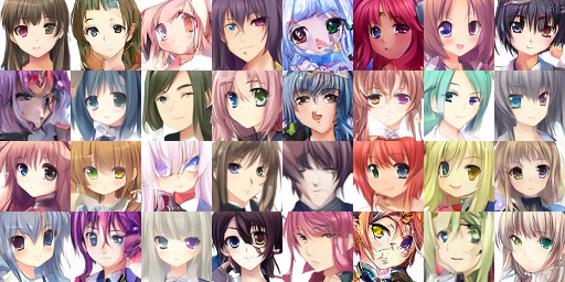
感觉总体上采样效果比 DDPM 稍微有所下降,不过也还在可以接受的范围内,算是一种速度-质量的 tradeoff。
语义插值效应复现
语义插值效应也比较简单,只需要修改初始化的 \(\mathbf{x}_T\) 即可。根据上文的叙述,我们首先实现球面线性插值: \[ \mathbf{x}_T^{(\alpha)}=\frac{\sin(1-\alpha)\theta}{\sin\theta}\mathbf{x}_T^{(0)}+\frac{\sin\alpha\theta}{\sin\theta}\mathbf{x}_T^{(1)},~~\mathrm{where}~\theta=\arccos\left(\frac{(\mathbf{x}_T^{(0)})^T\mathbf{x}_T^{(1)}}{||\mathbf{x}_T^{(0)}||~||\mathbf{x}_T^{(1)}||}\right) \]
1 | import torch |
我们这次要实现的和原论文不同,原论文的插值只在一行内部,我们希望实现一个二维的插值,也就是在一个图片网格中,从左上角到右下角存在一个渐变效果。为此,我们需要先构建一个二维的图片网格,然后按以下的步骤完成二维插值:
- 初始化网格四角的 \(\mathbf{x}_T\sim\mathcal{N}(0,1)\);
- 在网格的最左侧和最右侧两列中进行插值,例如最左侧的一列由左上角与左下角两个样本插值得到、最右侧的一列由右上角与右下角的两个样本插值得到;
- 遍历所有行,把每行中间的元素用该行最左侧与最右侧的元素进行插值,完成全部 \(\mathbf{x}_T\) 的初始化。
具体的直接看代码就好:
1 | def interpolation_grid( |
最后把 images 的初始化从 torch.randn
改成调用 interpolation_grid:
1 | images = interpolation_grid(rows, cols, in_channels, sample_size).to(unet.device) |
看一下结果如何:
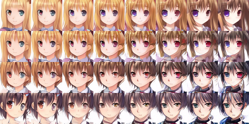
感觉还不错,那么 DDIM 的学习到这里就告一段落了。
总结
感觉 DDIM 还是非常神奇的,通过改变推导方式去除了对马尔可夫假设的依赖,而且最后表达式中几个复杂的项相互都可以消掉,最后得到一个比较优美的结果。而且最重要的是采样速度真的变快了好多,也因此我直接把实验从集群上搬到了我自己的 PC 上,的确很高效。
本文的代码在如下的链接中,后续还会更新更多 diffusion models 相关的文章,欢迎追更:
- 完整代码:https://github.com/LittleNyima/code-snippets/tree/master/ddim-tutorial
- 模型权重:https://huggingface.co/LittleNyima/ddpm-anime-faces-64
参考资料: