笔记|扩散模型(一)DDPM 理论与实现
感谢 qq、wbs、hsh 等读者对本文提出的宝贵意见(大拍手
端午假期卷一卷,开一个新坑系统性地整理一下扩散模型的相关知识。扩散模型的名字来源于物理中的扩散过程,对于一张图像来说,类比扩散过程,向这张图像逐渐加入高斯噪声,当加入的次数足够多的时候,图像中像素的分布也会逐渐变成一个高斯分布。当然这个过程也可以反过来,如果我们设计一个神经网络,每次能够从图像中去掉一个高斯噪声,那么最后就能从一个高斯噪声得到一张图像。虽然一张有意义的图像不容易获得,但高斯噪声很容易采样,如果能实现这个逆过程,就能实现图像的生成。
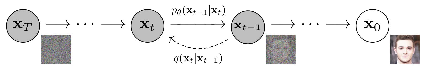
这个过程可以形象地用上图表示,扩散模型中有两个过程,分别是前向过程(从图像加噪得到噪音)和反向过程(从噪音去噪得到图像)。在上图中,向图像 \(\mathbf{x}_0\) 逐渐添加噪声可以得到一系列的 \(\mathbf{x}_1,\mathbf{x}_2,...,\mathbf{x}_T\),最后的 \(\mathbf{x}_T\) 即接近完全的高斯噪声,这个过程显然是比较容易的。而从 \(\mathbf{x}_T\) 逐渐去噪得到 \(\mathbf{x}_0\) 并不容易,扩散模型学习的就是这个去噪的过程。
前向过程
我们从比较简单的前向过程开始,第一个问题是如何向图像中添加高斯噪声。在 DDPM 中,加噪的方式是直接对图像和标准高斯噪声 \(\epsilon_{t-1}\sim\mathcal{N}(0,\mathbf{I})\) 进行加权求和: \[ \mathbf{x}_{t}=\sqrt{1-\beta_t}\mathbf{x}_{t-1}+\sqrt{\beta_t}\epsilon_{t-1} \] 这里的 \(\beta_t\) 就是每一步加噪使用的方差,在实际上进行加噪时,起始时使用的方差比较小,随着加噪步骤增加,方差会逐渐增大。例如在 DDPM 的原文中,使用的方差是从 \(\beta_1=10^{-4}\) 随加噪时间步线性增大到 \(\beta_T=0.02\)。这样设置主要是为了方便模型进行学习,如果在最开始就加入很大的噪声,对图像信息的破坏会比较严重,不利于模型学习图像的信息。这个过程也可以从反向进行理解,即去噪时先去掉比较大的噪音得到图像的雏形,再去掉小噪音进行细节的微调。
在上边的公式里,我们可以认为 \(\mathbf{x}_t\) 满足均值为 \(\sqrt{1-\beta_t}\mathbf{x}_{t-1}\),标准差为 \(\sqrt{\beta_t}\mathbf{I}\) 的高斯分布。这样可以把上述加权求和的过程写成条件概率分布的形式: \[ q(\mathbf{x}_t|\mathbf{x}_{t-1})=\mathcal{N}(\mathbf{x}_t;\sqrt{1-\beta_t}\mathbf{x}_{t-1},\beta_t\mathbf{I}) \] 上边等号的右边表示的就是当前的变量 \(\mathbf{x}_t\) 满足一个 \(\mathcal{N}(\sqrt{1-\beta_t}\mathbf{x}_{t-1},\beta_t\mathbf{I})\) 的概率分布。通过上边的公式我们可以看到,每一个时间步的 \(\mathbf{x}_t\) 都只和 \(\mathbf{x}_{t-1}\) 有关,因此这个扩散过程是一个马尔可夫过程。在前向过程中,每一步的 \(\beta\) 都是固定的,真正的变量只有 \(\mathbf{x}_{t-1}\),那么我们可以将公式中的 \(\mathbf{x}_{t-1}\) 进一步展开: \[ \begin{aligned} \mathbf{x}_t&=\sqrt{1-\beta_t}\mathbf{x}_{t-1}+\sqrt{\beta_t}\epsilon_{t-1}\\ &=\sqrt{1-\beta_t}(\sqrt{1-\beta_{t-1}}\mathbf{x}_{t-2}+\sqrt{\beta_{t-1}}\epsilon_{t-2})+\sqrt{\beta_t}\epsilon_{t-1}\\ &=\sqrt{(1-\beta_t)(1-\beta_{t-1})}\mathbf{x}_{t-2}+\sqrt{(1-\beta_t)\beta_{t-1}}\epsilon_{t-2}+\sqrt{\beta_t}\epsilon_{t-1} \end{aligned} \] 在上边的公式里,实际上 \(\epsilon_{t-2}\) 和 \(\epsilon_{t-1}\) 是同分布的,都是 \(\mathcal{N}(0,1)\),因此可以进行合并: \[ \begin{aligned} \mathbf{x}_t&=\sqrt{(1-\beta_t)(1-\beta_{t-1})}\mathbf{x}_{t-2}+\sqrt{(\sqrt{(1-\beta_t)\beta_{t-1}})^2+(\sqrt{\beta_t})^2}\bar{\epsilon}_{t-2}\\ &=\sqrt{(1-\beta_t)(1-\beta_{t-1})}\mathbf{x}_{t-2}+\sqrt{1-(1-\beta_t)(1-\beta_{t-1})}\bar{\epsilon}_{t-2} \end{aligned} \] 令 \(\alpha_t=1-\beta_t\),\(\bar{\alpha}_t=\prod_{i=1}^t\alpha_i\),继续推导,可以得到: \[ \begin{aligned} \mathbf{x}_t&=\sqrt{\alpha_t\alpha_{t-1}}\mathbf{x}_{t-2}+\sqrt{1-\alpha_t\alpha_{t-1}}\bar{\epsilon}_{t-2}\\ &=\cdots\\ &=\sqrt{\bar{\alpha}_t}\mathbf{x}_0+\sqrt{1-\bar{\alpha}_t}\epsilon \end{aligned} \] 通过上述的推导,我们发现给定 \(\mathbf{x}_0\) 和加噪的时间步,可以直接用一步就得到 \(\mathbf{x}_t\),而并不需要一步步地重复最开始的加权求和。和上述同理,这个关系也可以写成: \[ q(\mathbf{x}_t|\mathbf{x}_0)=\mathcal{N}(\mathbf{x}_t;\sqrt{\bar{\alpha}_t}\mathbf{x}_0,(1-\bar{\alpha}_t)\mathbf{I}) \] 从这个式子里我们可以看出,加噪过程中的 \(\mathbf{x}_t\) 可以看作原始图像 \(\mathbf{x}_0\) 和高斯噪声 \(\epsilon\) 的线性组合,且两个组合系数的平方和为 1。在实现加噪过程时,加噪的 scheduler 也是根据 \(\bar{\alpha}_t\) 设计的,这样更加直接,且为了保证最后得到的足够接近噪声,可以将 \(\bar\alpha_t\) 直接设置为一个接近 0 的数。
反向过程
正如文章开始所说的,反向过程就是从 \(\mathbf{x}_T\) 逐渐去噪得到 \(\mathbf{x}_0\) 的过程,也就是求 \(q(\mathbf{x}_{t-1}|\mathbf{x}_t)\)。根据贝叶斯公式: \[ q(\mathbf{x}_{t-1}|\mathbf{x}_t)=\frac{q(\mathbf{x}_t|\mathbf{x}_{t-1})q(\mathbf{x}_{t-1})}{q(\mathbf{x}_t)} \] 在上边的公式里,在前文中我们已经给出了 \(q(\mathbf{x}|\mathbf{x}_{t-1})\),但 \(q(\mathbf{x}_{t-1})\) 和 \(q(\mathbf{x}_t)\) 依然是未知的。虽然这两个分布目前未知,但是在上一节的最后,我们已经推导出了 \(q(\mathbf{x}_t|\mathbf{x}_0)\) 这个分布,那么我们可以给上面的贝叶斯公式加上 \(\mathbf{x}_0\) 作为条件,将等号右侧的两个未知分布转化为已知分布: \[ q(\mathbf{x}_{t-1}|\mathbf{x}_t,\mathbf{x}_0)=\frac{q(\mathbf{x}_t|\mathbf{x}_{t-1},\mathbf{x}_0)q(\mathbf{x}_{t-1}|\mathbf{x}_0)}{q(\mathbf{x}_t|\mathbf{x}_0)} \] 而且因为先验分布 \(q(\mathbf{x}_t|\mathbf{x}_{t-1})\) 是马尔可夫过程,\(\mathbf{x}_t\) 只与 \(\mathbf{x}_{t-1}\) 有关,而与 \(\mathbf{x}_0\) 无关,所以上边式子里的 \(q(\mathbf{x}_t|\mathbf{x}_{t-1},\mathbf{x}_0)=q(\mathbf{x}_t|\mathbf{x}_{t-1})\)。但推导到这里还有问题,我们把 \(\mathbf{x}_0\) 加入到了条件概率分布的条件中,但 \(\mathbf{x}_0\) 依然是未知的,因此我们需要继续推导出一个与 \(\mathbf{x}_0\) 无关的式子。
上面的公式右侧的几个条件概率分布全都是高斯分布: \[ \begin{aligned} q(\mathbf{x}_t|\mathbf{x}_{t-1})&=\mathcal{N}(\mathbf{x}_t;\sqrt{\alpha_t}\mathbf{x}_{t-1},1-\alpha_t)\\ q(\mathbf{x}_{t-1}|\mathbf{x}_0)&=\mathcal{N}(\mathbf{x}_{t-1};\sqrt{\bar{\alpha}_{t-1}}\mathbf{x}_0,1-\bar{\alpha}_{t-1})\\ q(\mathbf{x}_t|\mathbf{x}_0)&=\mathcal{N}(\mathbf{x}_t;\sqrt{\bar{\alpha}_t}\mathbf{x}_0,1-\bar\alpha_t) \end{aligned} \] 用概率密度函数把这个公式展开,如果不看前边的常数项,可以得到: \[ \begin{aligned} q(\mathbf{x}_{t-1}|\mathbf{x}_t,\mathbf{x}_0)&\propto\exp\left(-\frac{1}{2}\left[\frac{(\mathbf{x}_t-\sqrt{\alpha_t}\mathbf{x}_{t-1})^2}{\beta_t}+\frac{(\mathbf{x}_{t-1}-\sqrt{\bar\alpha_{t-1}}\mathbf{x}_0)^2}{1-\bar\alpha_{t-1}}+\frac{(\mathbf{x}_t-\sqrt{\bar{\alpha}_t}\mathbf{x}_0)}{1-\bar\alpha_t}\right]\right)\\ \end{aligned} \] 因为我们在这一步去噪的时候想求得的是 \(\mathbf{x}_{t-1}\) 的分布,所以我们把上式展开并整理成一个关于 \(\mathbf{x}_{t-1}\) 的多项式: \[ q(\mathbf{x}_{t-1}|\mathbf{x}_t,\mathbf{x}_0)\propto\exp\left(-\frac{1}{2}\left[\left(\frac{\alpha_t}{\beta_t}+\frac{1}{1-\bar\alpha_{t-1}}\right)\mathbf{x}_{t-1}^2-\left(\frac{2\sqrt{\alpha_t}}{\beta_t}\mathbf{x}_t+\frac{2\sqrt{\bar\alpha_{t-1}}}{1-\bar\alpha_{t-1}}\mathbf{x}_0\right)\mathbf{x}_{t-1}+C(\mathbf{x}_t,\mathbf{x}_0)\right]\right) \] 上边的式子里常数项不重要(因为可以直接变成常数从指数部分挪走),所以可以暂时不管。对比高斯分布(可以证明反向过程的分布也是高斯分布)的指数部分 \(\exp\left(-\frac{1}{2}\left(\frac{1}{\sigma^2}x^2-\frac{2\mu}{\sigma^2}x+\frac{\mu^2}{\sigma^2}\right)\right)\): \[ \begin{cases} \begin{aligned} \frac{1}{\sigma^2}&=\frac{\alpha_t}{\beta_t}+\frac{1}{1-\bar\alpha_{t-1}}\\ \frac{2\mu}{\sigma^2}&=\frac{2\sqrt{\alpha_t}}{\beta_t}\mathbf{x}_t+\frac{2\sqrt{\bar\alpha_{t-1}}}{1-\bar\alpha_{t-1}}\mathbf{x}_0 \end{aligned} \end{cases} \] 可以发现 \(\sigma\) 的表达式里都是我们 scheduler 里的定值,而求解出均值 \(\mu\): \[ \mu=\frac{\sqrt{\alpha_t}(1-\bar\alpha_{t-1})}{1-\bar\alpha_t}\mathbf{x}_t+\frac{\sqrt{\bar\alpha_{t-1}}\beta_t}{1-\bar\alpha_t}\mathbf{x}_0 \] 代入上一章最后的 \(\mathbf{x}_t=\sqrt{\bar{\alpha}_t}\mathbf{x}_0+\sqrt{1-\bar{\alpha}_t}\epsilon\),得到: \[ \mu=\frac{1}{\sqrt{\alpha_t}}\left(\mathbf{x}_t-\frac{1-\alpha_t}{\sqrt{1-\bar\alpha_t}}\tilde{\epsilon}\right) \] 注意在反向过程中我们并不知道在前向过程中加入的噪声 \(\epsilon\) 是 \(\mathcal{N}(0,1)\) 中的具体哪一个噪声,而噪声也没有办法继续转换成其他的形式。因此我们使用神经网络在反向过程中估计的目标就是 \(\tilde{\epsilon}\)。在这个网络中,输入除了 \(\mathbf{x}_t\) 之外还需要 \(t\),可以简单理解为:加噪过程中 \(\mathbf{x}_t\) 的噪声含量是由 \(t\) 决定的,因此在预测噪声时也需要知道时间步 \(t\) 作为参考,以降低预测噪声的难度。
注:关于反向过程为什么要这样做,Lilian Weng 基于变分推断给出了一个复杂的证明,因为过于难以理解,这里暂且把它跳过。(以后有可能会填坑,也有可能不会x)
具体的训练过程
我们已经知道了去噪网络的参数和预测目标,下一个问题就是如何去训练这个去噪网络。原始论文中给出了如下的训练过程:
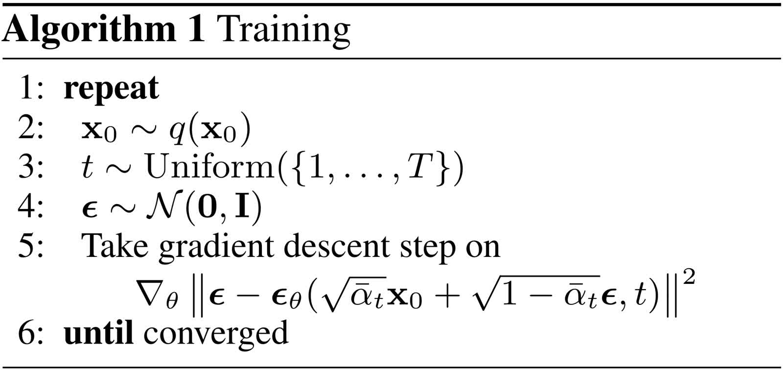
在上面的算法中,首先从数据集 \(q(\mathbf{x}_0)\) 中采样出 \(\mathbf{x}_0\),从 1 到 T 的均匀分布中采样出 \(t\),从标准高斯分布中采样出 \(\epsilon\)。然后根据 \(\mathbf{x}_t=\sqrt{\bar{\alpha}_t}\mathbf{x}_0+\sqrt{1-\bar{\alpha}_t}\epsilon\) 将 \(\mathbf{x}_0\) 与 \(\epsilon\) 加权求和得到噪声图,最后将噪声图和时间步输入到网络中预测噪声,并用真实的噪声计算出 L2 损失进行优化。
这里比较难理解的是 \(\epsilon\) 本身就是从标准高斯分布中采样出的,为什么还需要一个网络专门对其进行预测。我个人的理解是:尽管每次添加的噪声都是从固定的分布中采样出的,但如果用同一个分布中的另一个采样出的样本将其代替,就会向去噪过程引入一定的误差,最后这些误差积累的结果会破坏最终生成的图像。
具体的采样过程
论文中同样也给出了采样过程:
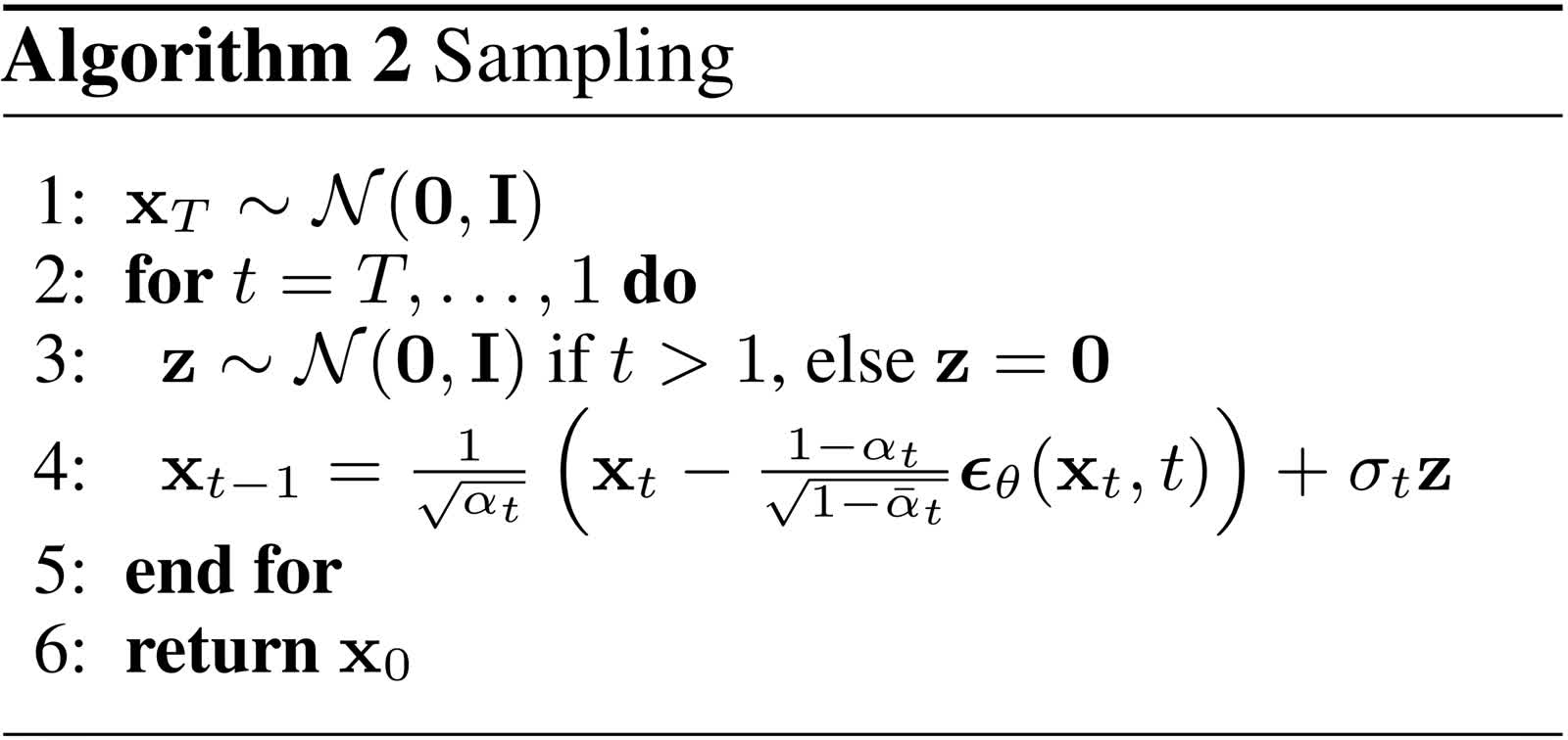
具体来说,首先从标准正态分布中采样出 \(\mathbf{x}_T\) 作为初始的图像,然后重复 \(T\) 步去噪过程。在每一步去噪过程中,由于我们已经推导出: \[ q(\mathbf{x}_{t-1}|\mathbf{x}_t)=\mathcal{N}\left(\mathbf{x}_{t-1};\frac{1}{\sqrt{\alpha_t}}\left(\mathbf{x}_t-\frac{1-\alpha_t}{\sqrt{1-\bar\alpha_t}}\tilde{\epsilon}\right),\sigma_t^2\right) \] 利用一个重参数化技巧:从 \(\mathcal{N}(\mu,\sigma^2)\) 采样可以实现为从 \(\mathcal{N}(0,1)\) 采样出 \(\epsilon\),再计算 \(\mu+\epsilon\cdot\sigma\)。这样即可实现从上述的高斯分布中采样出 \(\mathbf{x}_{t-1}\)。如此重复 \(T\) 次即可得到最终的结果,注意最后一步的时候没有采样,而是只加上了均值。
DDPM 的代码实现
现有的主流方法使用 UNet 来实现去噪网络,如下图所示。
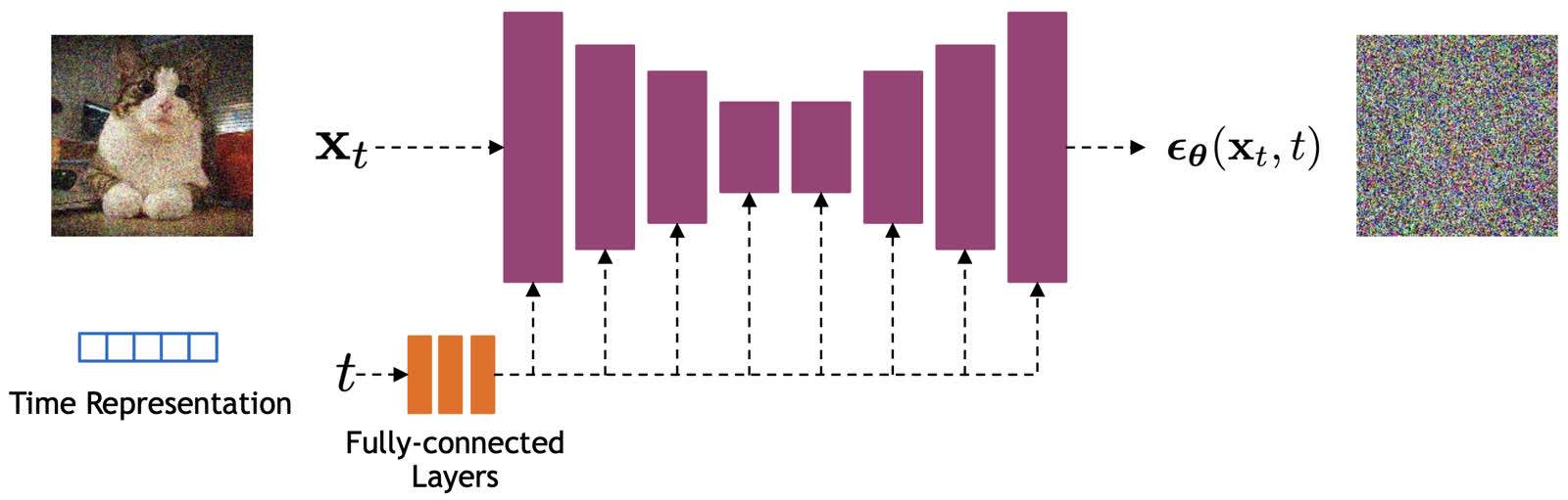
为了降低理解的难度,我们这里不关心这个去噪网络的具体实现,只需要知道这个网络接收一个噪声图
\(\mathbf{x}_t\) 和一个时间步 \(t\) 作为参数,并输出一个噪声的预测结果
\(\epsilon_\theta(\mathbf{x}_t,t)\)。在
diffusers 库中已经实现了一个 2D UNet
网络,我们直接使用即可。下面我们也主要使用 diffusers 实现
DDPM 模型。
训练参数
首先配置训练的参数:
1 | from dataclasses import dataclass |
训练数据
我们使用 huggan/anime-faces 数据集,这个数据集由 21551
张分辨率为 64x64 的动漫人物头像组成。我们加载这个数据集:
1 | from datasets import load_dataset |
由于这个数据集的作者组织数据的方式不太规范,所以最后加载进来实际上数据集的长度是 86204,也就是 21551 张图片每张重复了 4 次,我们只需要保留前 21551 个样本即可。
然后为数据集设置预处理函数:
1 | from torchvision import transforms |
最后创建 dataloader:
1 | from torch.utils.data import DataLoader |
降噪网络
我们可以直接用 diffusers 创建降噪网络:
1 | from diffusers import UNet2DModel |
核心代码
前边的三个部分分别配置了一些训练参数,以及训练数据和模型,这些都是比较工程化的部分,而我们在上面推导的 DDPM 核心算法还没有实现。在这一小节我们主要来实现核心的算法。
首先我们需要先定义 \(\beta\)、\(\alpha\),以及 \(\bar\alpha\) 等最基本的常量,这里我们保持 DDPM 原论文的配置,也就是 \(\beta\) 初始为 \(1\times10^{-4}\),最终为 \(0.02\),且共有 \(1000\) 个时间步:
1 | import torch |
然后是比较简单的前向过程,只需要实现加噪即可,按照 \(\mathbf{x}_t=\sqrt{\bar{\alpha}_t}\mathbf{x}_0+\sqrt{1-\bar{\alpha}_t}\epsilon\) 这个公式实现即可。注意需要将系数的维度数量都与输入样本对齐:
1 | class DDPM: |
反向过程相对来说比较复杂,不过因为我们已经完成了公式的推导,只需要按照公式实现即可。我们也再把公式贴到这里,对着公式实现具体的代码: \[ \begin{aligned} \sigma&=\left(\frac{\alpha_t}{\beta_t}+\frac{1}{1-\bar\alpha_{t-1}}\right)^{-1/2}\\ \mu&=\frac{1}{\sqrt{\alpha_t}}\left(\mathbf{x}_t-\frac{1-\alpha_t}{\sqrt{1-\bar\alpha_t}}\tilde{\epsilon}_t\right) \end{aligned} \]
1 | class DDPM: |
训练与推理
最后是训练和推理的代码,这部分也比较工程,直接套用现成代码即可:
1 | from accelerate import Accelerator |
结果展示
训练在一张 NVIDIA GeForce RTX 4090 GPU 上大概需要运行 3 个多小时,最后的结果大概长这个样子:
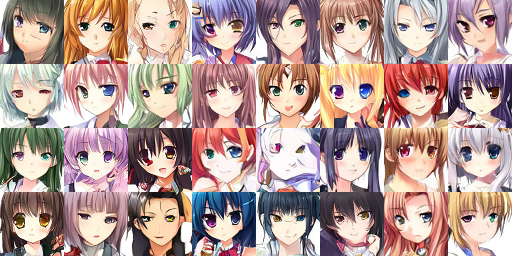
可以看到虽然里边难免有一些比较奇形怪状的结果,不过总体上来说已经初具雏形了。
总结
本文总结了 DDPM 的理论和实现方式,在代码部分我们是完全根据推导出的公式实现的采样过程。实际上在很多代码库中,采样过程并没有严格按照论文中的公式实现,而是先从 \(\mathbf{x}_t\)、\(t\) 和预测的噪声反向计算出 \(\mathbf{x}_0\),再基于 \(\mu=\frac{\sqrt{\alpha_t}(1-\bar\alpha_{t-1})}{1-\bar\alpha_t}\mathbf{x}_t+\frac{\sqrt{\bar\alpha_{t-1}}\beta_t}{1-\bar\alpha_t}\mathbf{x}_0\) 计算均值,这样的好处在于可以对 \(\mathbf{x}_0\) 进一步规范化,控制输出的范围。
可以看出 DDPM 虽然理论比较复杂,但实现起来还是比较简单直接的。因为作者本人对 diffusion models 的理解也不算非常深入,所以如果文章有问题的话欢迎各位读者来讨论,后续(如果没有鸽掉的话)还会更新一些其他的 diffusion models 的文章,欢迎追更)
本文完整的代码以及训练好的模型见如下链接:
- 完整代码:https://github.com/LittleNyima/code-snippets/tree/master/ddpm-tutorial
- 模型权重:https://huggingface.co/LittleNyima/ddpm-anime-faces-64
参考资料: